The first post in this series is here. The previous post in this series is here. The next post in this series is here.
If you are into the latest language tech innovations, you very likely came across the notion of a neural network. You probably also heard of a machine and deep learning. Maybe you are even considering larger deployment of these technologies in your organization?
To add a bit of an explanatory touch to our texts, we started a mini-series, in which we explain scientific foundations of those technologies for those, who have little prior knowledge. We have already explained what a neuron is and how it makes connections in Part One and what does the neural network really ‘do’ in Part Two.
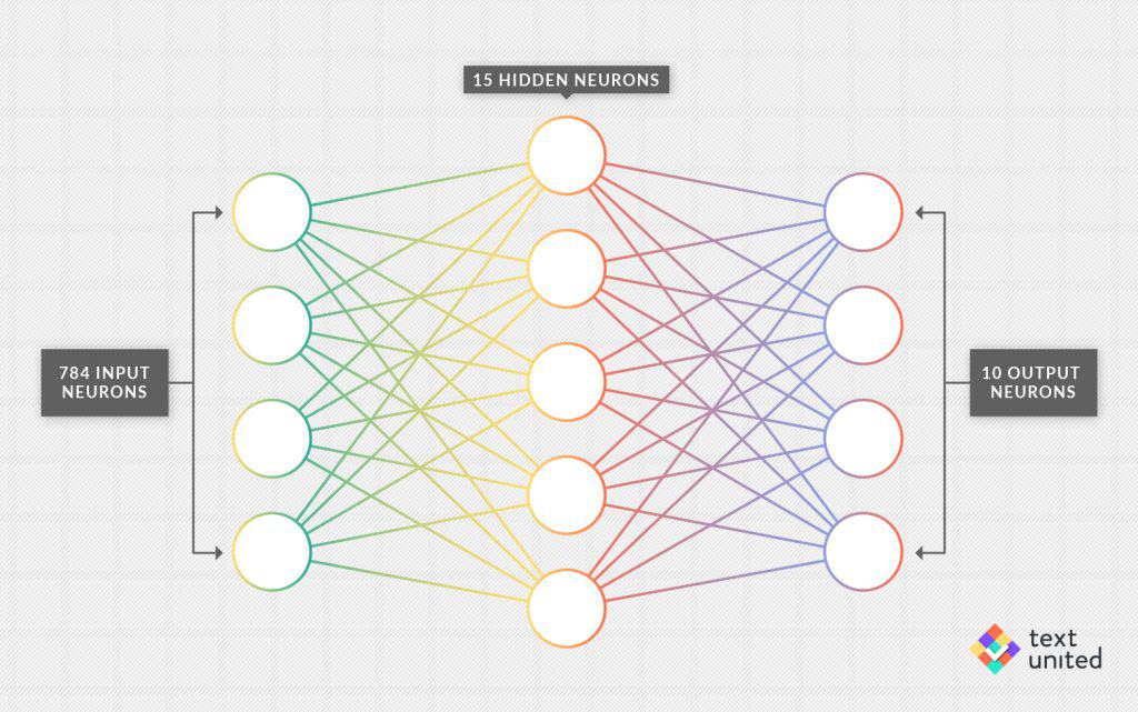
Today we will finally take a look at how machines ‘learn’. Last time we built a simple neural network with one hidden layer, which was designed to read handwritten digits.
However, we still had roughly 12.000 parameters which had to be initialized. Choosing that many parameters in the right way seems to be a daunting task. Let’s just initialize them to be completely random numbers from some given distribution. Now when we plug in a picture of a handwritten digit (say, seven), we obviously get a meaningless output in the form of ten numbers. Of course, we would like the seventh output neuron to light up, while all the others should be negligible.
To make progress we have to tell our network what we want it to do, given some input. We do this by introducing a so-called ‘training data’. In our case, this training data is a set of digital images of handwritten numbers, together with a description of the underlying number. Quite often a lot of work has to go into such a training data, as the ability to distinguish handwritten digits (or translating text) needs to ultimately come from a human being. Luckily, in the case of handwritten digits, there is an online database called ‘MNIST’ of 60.000 images of the right file size plus a list of the underlying numbers.
The next step is to measure how well our neural network is doing on this training set. We need to introduce a so-called cost-function. It will usually have the form of a very big sum, with one term per training example (so in our case, a sum with 60.000 terms). So for each digital image, there is a term in the cost-function, which depends on the actual number that is being depicted and the output of our neural network given that input. We will call such terms ‘error-terms’. There is some freedom as to how to choose the error-terms.
The main requirement is that when the neural network is having an output close to what is required, the corresponding error-term in the cost-function should be small. Otherwise, it should be large. Imagine that one of the training examples is a handwritten two, but the output neuron corresponding to the number seven has the strongest activation. Then, the error-term corresponding to this training example should be large. If however, only the correct output neuron would light up, then the same error-term should be small or even equal to zero. The cost-function being the sum of all error-terms, then measures the overall performance of the neural network.
Now imagine, that every time your neural network makes a mistake you have to pay the error-term. Then the cost-function would be just the overall cost, and hence the name. So the cost-function measures how well our neural network is performing. A small cost-function means the network does a good job, while a large one means that it does a bad job.
If that is the only thing you understood from this paragraph, then you are perfectly fine as this will be the only thing we will need to understand the next post of this series!

