The first post in this series is here. The previous post in this series is here. The next post in this series is here.
Welcome back to the series where we explain scientific foundations of neural network technologies to dive into their use of natural language processing and neural machine translation. The purpose of all that is to really show you what is going on behind the curtain.
In part seven we have explored various ways in which semantic relations are encoded in the linear structure of word vectors. We’ve mentioned that this idea was studied using a neural network algorithm called ‘Word2vec’ introduced by Mikolov et al. in the papers ‘Distributed Representations of Words and Phrases and their Compositionality’ and ‘Efficient Estimation of Word Representations in Vector Space’ back in 2013.
In the first part of today’s blog, we’ll get a little bit more quantitative about the accuracy of the word analogy task introduced last time and in the second, take a closer look at the implementation of Word2Vec. It is a nice way to refresh your memory of the concepts we have encountered in earlier blogs.
The Accuracy of Word Analogy Task
Last time we have seen two different ways in which the linear structure of word vectors was useful (when I say ‘linear structure’, I just mean the fact that vectors can be added).
One was given by simple addition and our prime example was:
vec(‘Germany’) + vec(‘capital’) = vec(‘Berlin’)
The other was an analogy reasoning task of the form
‘a is to b as c is to d’
where one of the letters is unknown.
Our example was
‘Madrid’ is to ‘Spain’ as ‘Paris’ is to ‘France’
which led the equation
vec(‘Madrid’) – vec(‘Spain’) = vec(‘Paris’) – vec(‘France’)
We will concentrate on the latter task.
First of all, let me mention that there are two implementations of Word2vec:
#1. ‘Continuous Bag-of-Words’ (or CBOW)
and
#2. ‘Skip-gram’
I’m going to explain what they do later, but for now, we’ll take them for granted. Next, we will need to talk about word vectors. The word vectors were trained using Google News corpus containing about 6 billion tokens. The vocabulary was constrained to the one million most frequent words.
The dimensionality of the word vectors, which is a hyperparameter, was varied between 50 and 600 dimensions. The performance on the Semantic-Syntactic Word Relationship test set, which I will explain in a moment, improved with higher dimensions, but saturated unless the training data was also enlarged. Hence, increasing the size of word vectors is only advantageous with a corresponding increase of training data.
What is Semantic-Syntactic Word Relationship Test Set?
In short, it’s an analogy test of the form
‘a’ is to ‘b’ as ‘c’ is to ‘_’
which is also abbreviated as
‘a:b::c:_’ (the blank stands for the word that has to be guessed)
The examples were from five different semantic categories like
‘Currency’ (USA:Dollar::Japan:Yen)
or
‘Man-Woman’ (brother:sister::grandson:granddaughter)
There are further nine syntactic categories, like
‘Opposite’ (possibly:impossibly::ethical:unethical)
or
‘Past tense’ (walking:walked::swimming:swam)
Overall there were 8869 semantic questions and 10675 syntactic ones.
How Did the Neural Network Perform?
On the semantic task, CBOW had 24% accuracy and Skip-gram had 55%. When it comes to syntactic questions, CBOW outperformed Skip-gram by 64% to 59%. In all cases, the performance was improved compared to the benchmark at that time. It is very interesting to note that depending on the task different models had different accuracies. That means that word vectors might have to be chosen task-specific.
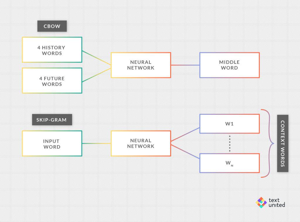
Finally, let me say something about architecture. I have mentioned two, namely Continuous Bag-of-Words and Skip-gram. For the first one, the idea is that for a given word (so-called ‘middle word’) in the training corpus one looks at the four words before it (‘history words’) and four words after it (‘future words’). Now, we take the average (the ‘bag-of-words’) of the corresponding 8-word vectors as the input to the neural network. Remember that these vectors are not given a priori, but rather, must be learned. The goal is to predict the middle word.
It is surprisingly difficult to implement an output layer, which needs an acceptable amount of computation and I will just mention that it involves the scalar product that we have seen last time. The Skip-gram works quite analogously. The only major difference is that this time the input is just one word, and the goal is to predict surrounding words.
I will leave you with some more examples of word analogy used in the experiments. To be honest and fair, I have also included a few wrong ones. Interestingly, it is not always clear what the right or wrong answer should be:
copper:Cu :: Zinc:Zn
Einstein:scientist :: Mozart:violinist
Berlusconi:Silvio :: Sarkozy:Nicolas
Japan:sushi :: USA:pizza
Microsoft:Windows :: IBM:Linux
Miami:Florida :: Dallas:Texas
Apple:Jobs :: Google:Yahoo
Next time we’ll return to linear algebra and introduce a new powerful concept, which is directly applicable for machine translation.
Stay Tuned!

