The first post in this series is here. The previous post in this series is here. The next post in this series is here.
Hey there! If you’re new here, let us explain that we started a mini-series, in which we explain the scientific foundations of neural network technologies. All that to explain what a Neural Network actually is, then dive into their use of natural language processing and consecutively, neural machine translation. The purpose of all that is to really show you what is going on behind the curtain.
In Part Four we explained the notion of a cost function. In this part, we will explore a new neural architecture, which will help us in natural language processing tasks. We have not seen how neural networks can help us with machine translation yet. Today we will take the first step in this direction!
The Curse of Dimensionality
Let’s take a look at a predecessor of the neural approach to neural translation, namely statistical translation. As you know, languages are from a purely informational point of view much more structured than just random noise. Some words tend to be more frequent than others. There is a complex theory that goes back to 1940s Claude Shannon’s work, but we will focus only on extracting an obvious problem with the statistical approach from it, namely the ‘curse of dimensionality’.
Let’s assume that we start with a small vocabulary of 10.000 words. It might not seem like a lot, but now imagine that we look at all possible combinations of four words from our vocabulary. This results in a staggering number of 10^16 or ten quadrillion quadruples. Wow. That’s a lot. Most quadruples will obviously not show up at all, but you get the idea.
Now, imagine that you have the sentence ‘Dogs are my favorite pets’ in your corpus (the data that the system has used for statistical evaluation). Your statistical translation system might consider this to be a likely candidate for some translation. But imagine that the right translation would be ‘Cats are my favorite pets’, and that this sentence does not appear in the corpus. One word changed, and the sentence becomes from the point of view of the machine as unlikely as ‘Windows are my favorite pets.’.
The Problem of The Statistical Approach and How To Solve It
The problem of the statistical approach is that words are treated as abstract objects, without any semantics. What if the machine would know that ‘dogs’ and ‘cats’ are in some sense close to each other? It could ‘think’ that the sentence ‘Dogs are my favourite pets’ is exactly the same as ‘Cats are my favourite pets’ because substitution is justified by the similarity. This is, of course, a caricature of the real problem. The above sentences are so simple that they can be translated word by word of course, but it illustrates the shortcomings of statistical translation.
So what do we need? We need to represent words in a way that captures not just their co-occurrence frequencies, but also their semantic relations. And here neural networks enter the game. You might be surprised that the idea to use neural networks for this purpose is quite old, going back to 1986’s Rumelhart, Hinton and Williams paper. We will not touch on back-propagation, as it is a rather technical aspect of neural networks. It is ‘learning representations’ that will be of main interest. Let us give you the essential abstract:
We describe a new learning procedure, back-propagation, for networks of neuron-like units. The procedure repeatedly adjusts the weights of the connections in the network so as to minimize a measure of the difference between the actual output vector of the net and the desired output vector. As a result of the weight adjustments, internal ‘hidden’ units, which are not part of the input or output, come to represent important features of the task domain, and the regularities in the task are captured by the interactions of these units. The ability to create useful new features distinguishes back-propagation from earlier, simpler methods such as the perceptron-convergence procedure.
You might recognize the part concerning adjusting weights and minimizing a measure of the difference (error) from previous blogs. The new idea important for us is the use of hidden units (or neurons) to represent important features. I will explain what is meant by this in the today’s blog.
Use Hidden Units To Represent Important Features
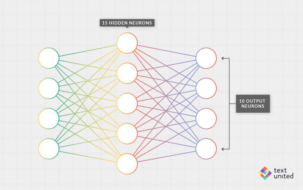
Remember the architecture of the neural network for recognizing handwritten digits? It had just one hidden layer consisting of 15 neurons:
Once the network gets quite good at its task, we might ask whether these 15 hidden neurons actually represent some particular features of the input. One neuron, for example, might represent a circle somewhere in the middle of the image, another one could fire when presented with a horizontal line. Given the predictive power of the network (more than 95 percent accuracy!), it seems reasonable. This idea is used in word representations, after all.
We will illustrate just one possible implementation, namely the skip-gram model. The input layer contains one neuron per word in the vocabulary. Having a particular word as the input is basically activating the corresponding neuron and we have one neuron per word in the vocabulary as the output. The task is, given a word as an input, output the distribution of words which co-occurs with the input. It sounds very much like statistical machine translation.
But What About The Hidden neurons? Here Is Where The Magic Happens!
Among the hidden layers, there will be one small, special layer, containing just 100 neurons. This might seem like a lot of neurons compared to the previous task of recognizing handwritten digits, where there were only 15. But with a task like the one above, hidden layers tend to be much larger. This ‘small’ hidden layer will play the role of a bottleneck. It means that any information which goes from the input to the output has to go through this 100-neuron hidden layer.
Think back to our earlier example of ‘dog’ and ‘cat’. Both words will co-occur with similar context words. Hence, once trained, they will also produce outputs, which are close to each other. That does not mean automatically that the hidden layers will also be similar. But the 100-neuron layer is, in fact, similar. Why? The size of the 100-neuron layer is so small that the network just cannot afford to have completely different activations in it while having similar outputs.
Remember, the input layer consists of a neuron for every word in our vocabulary. With a 100.000 words vocabulary, the number of neurons in the 100-neuron layer will be decreased 1000-fold as compared to the input layer. Clearly, a lot of smart data compression needs to happen, in order to still have meaningful results. Words with similar contexts will likely have similar activations in the 100-neuron layer.
The last ingenious step is taking the activation in the 100-neuron layer as a representation of the underlying word. From now on, we will call it a ‘word representation’. The hope is that these arrays or vectors of 100 numbers capture some semantic relations (similar words, having similar representations). In fact, it turns out that they capture far more semantic relations than just similarity. But this has to wait until the next blog 😉
Stay Tuned For More!

